
This blog is based on some exploratory data analysis performed on the corpora provided for the “Spooky Author Identification” challenge at Kaggle.
The Spooky Challenge
A Halloween-based challenge [1] with the following goal using data analysis: predict who was writing a sentence of a possible spooky story between Edgar Allan Poe, HP Lovecraft, and Mary Wollstonecraft Shelley.“Deep into that darkness peering, long I stood there, wondering, fearing, doubting, dreaming dreams no mortal ever dared to dream before." Edgar Allan Poe
“That is not dead which can eternal lie, And with strange eons, even death may die.” HP Lovecraft
“Life and death appeared to me ideal bounds, which I should first break through, and pour a torrent of light into our dark world.” Mary Wollstonecraft Shelley
The toolset for data analysis
The only tools available to us during this exploration will be our intuition, curiosity, and the selected packages for data analysis. Specifically:tidytextpackage, text mining for word processing, and sentiment analysis using tidy toolstidyversepackage, an opinionated collection of R packages designed for data sciencewordcloudpackage, pretty word cloudsgridExtrapackage, supporting functions to work withgridgraphicscaretpackage, supporting function for performing stratified random samplingcorrplotpackage, a graphical display of a correlation matrix, confidence interval
# Required libraries
if packages are not installed
install.packages(“packageName”)
library(tidytext)

library(tidyverse)

library(gridExtra)

library(wordcloud)

library(dplyr)

library(complot)
The beginning of the exploratory data analysis journey: The Spooky data
We are given a CSV file, the train.csv, containing some information about the authors. The information consists of a set of sentences written by different authors (EAP, HPL, MWS). Each entry (line) in the file is an observation providing the following information:an id, a unique id for the excerpt/ sentence (as a string) the text, the excerpt/ sentence (as a string), the author, the author of the excerpt/ sentence (as a string) - a categorical feature that can assume three possible values EAP for Edgar Allan Poe,
HPL for HP Lovecraft,
MWS for Mary Wollstonecraft Shelley
 # loading the data using readr package

  spooky_data <- readr::read_csv(file = "./../../../data/train.csv",

                    col_types = "ccc",

                    locale = locale("en"),

                    na = c("", "NA"))


  # readr::read_csv does not transform string into factor

  # as the "author" feature is categorical by nature

  # it is transformed into a factor

  spooky_data$author <- as.factor(spooky_data$author)
The overall data includes 19579 observations with 3 features (id, text, author). Specifically 7900 excerpts (40.35 %) of Edgard Allan Poe, 5635 excerpts (28.78 %) of HP Lovecraft, and 6044 excerpts (30.87 %) of Mary Wollstonecraft Shelley.
Read about Data Normalization in predictive modeling before analytics in this blog
Avoid the madness!
It is forbidden to use all of the provided spooky data for finding our way through the unique spookiness of each author.We still want to evaluate how our intuition generalizes on an unseen excerpt/sentence, right?
For this reason, the given training data is split into two parts (using stratified random sampling)
- an actual training dataset (70% of the excerpts/sentences), used for
- exploration and insight creation, and
- training the classification model
- a test dataset (the remaining 30% of the excerpts/sentences), used for
- evaluation of the accuracy of our model.
# setting the seed for reproducibility
set.seed(19711004)
trainIndex <- caret::createDataPartition(spooky_data$author, p = 0.7, list = FALSE, times = 1)
spooky_training <- spooky_data[trainIndex,]
spooky_testing <- spooky_data[-trainIndex,]
Is the provided data usable? Question: Does each observation have an id? An excerpt/sentence associated with it? An author?
missingValueSummary <- colSums(is.na(spooky_training))
Some initial facts about the excerpts/sentences
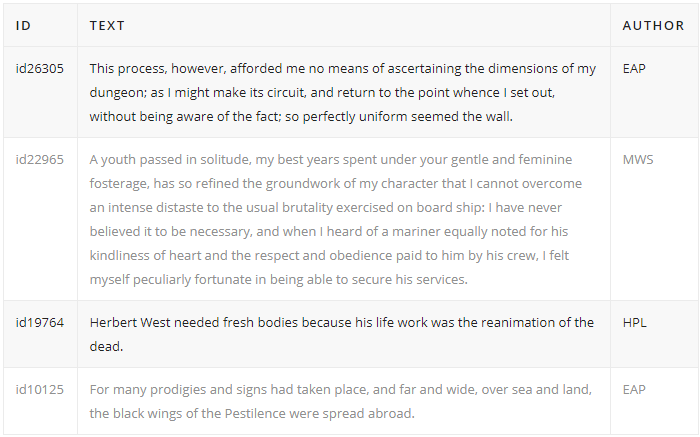
Below we can see, as an example, some of the observations (and excerpts/sentences) available in our dataset.
 EAP
EAP
Question: How many excerpts/sentences are available by the author?
no_excerpts_by_author <- spooky_training %>%
dplyr::group_by(author) %>%
dplyr::summarise(n = n())
ggplot(data = no_excerpts_by_author,
mapping = aes(x = author, y = n, fill = author)) +
geom_col(show.legend = F) +
ylab(label = "number of excerpts") +
theme_dark(base_size = 10)</code></pre>
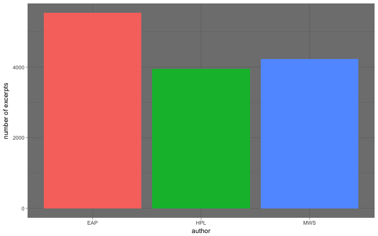 Number of excerpts mapped against author-name
Question: How long (# ofchars) are the excerpts/sentences by the author?
spooky_training$len <- nchar(spooky_training$text)
ggplot(data = spooky_training, mapping = aes(x = len, fill = author)) +
geom_histogram(binwidth = 50) +
facet_grid(. ~ author) +
xlab(“# of chars”) +
theme_dark(base_size = 10)
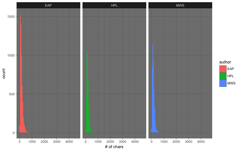 Count and number of characters graph
ggplot(data = spooky_training, mapping = aes(x = 1, y = len)) +
geom_boxplot(outlier.colour = "red", outlier.shape = 1) +
facet_grid(. ~ author) +
xlab(NULL) +
ylab("# of chars") +
theme_dark(base_size = 10)
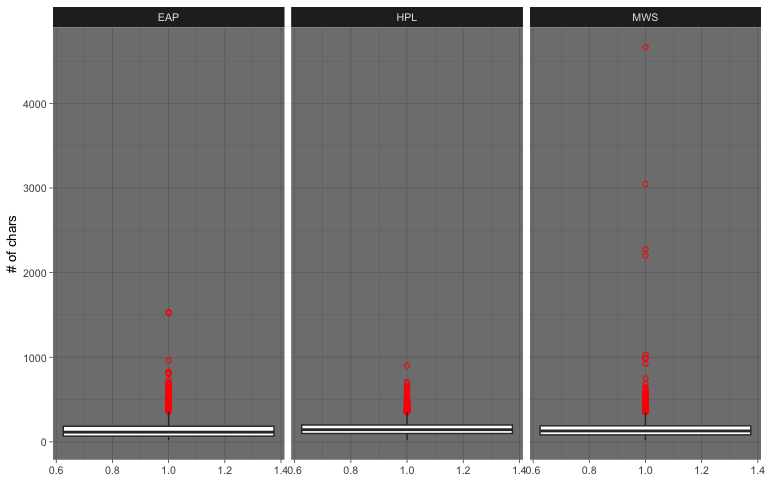 Number of characters
Some excerpts are very long. As we can see from the boxplot above, there are a few outliers for each author; a possible explanation is that the sentence segmentation has a few hiccups.
MWS) has an excerpt of around 4600 characters:Thinking Point: “What do we want to do with those excerpts/outliers?”
Some more facts about the excerpts/sentences using the bag-of-words
The data is transformed into a tidy format (unigrams only) to use the tidy tools to perform some basic and essential NLP operations.spooky_trainining_tidy_1n <- spooky_training %>%
select(id, text, author) %>%
tidytext::unnest_tokens(output = word,
input = text,
token = "words",
to_lower = TRUE)</code></pre>
Each sentence is tokenized into words (normalized to lower case, removed punctuation). See example below how the data (each excerpt/sentence) was and how it has been transformed.
Question: Which are the most common words used by each author?
Lets start to count how many times words has been used by each author and plot.
words_author_1 <- plot_common_words_by_author(x = spooky_trainining_tidy_1n,
author = "EAP",
greater.than = 500)
words_author_2 <- plot_common_words_by_author(x = spooky_trainining_tidy_1n,
author = "HPL",
greater.than = 500)
words_author_3 <- plot_common_words_by_author(x = spooky_trainining_tidy_1n,
author = "MWS",
greater.than = 500)
gridExtra::grid.arrange(words_author_1, words_author_2, words_author_3, nrow = 1)
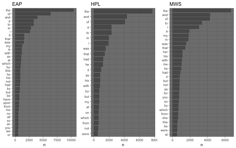 Most common words used by each author
From this initial visualization we can see that the authors use quite often the same set of words - like the, and, of. These words do not give any actual information about the vocabulary actually used by each author, they are common words that represent just noise when working with unigrams: they are usually called stopwords.
If the stopwords are removed, using the list of stopwords provided by the tidytext package, it is possible to see that the authors do actually use different words more frequently than others (and it differs from author to author, the author vocabulary footprint).
words_author_1 <- plot_common_words_by_author(x = spooky_trainining_tidy_1n,
author = "EAP",
greater.than = 70,
remove.stopwords = T)
words_author_2 <- plot_common_words_by_author(x = spooky_trainining_tidy_1n,
author = "HPL",
greater.than = 70,
remove.stopwords = T)
words_author_3 <- plot_common_words_by_author(x = spooky_trainining_tidy_1n,
author = "MWS",
greater.than = 70,
remove.stopwords = T)
gridExtra::grid.arrange(words_author_1, words_author_2, words_author_3, nrow = 1)
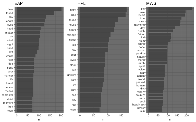 Most common words used comparison between EAP, HPL, and MWS
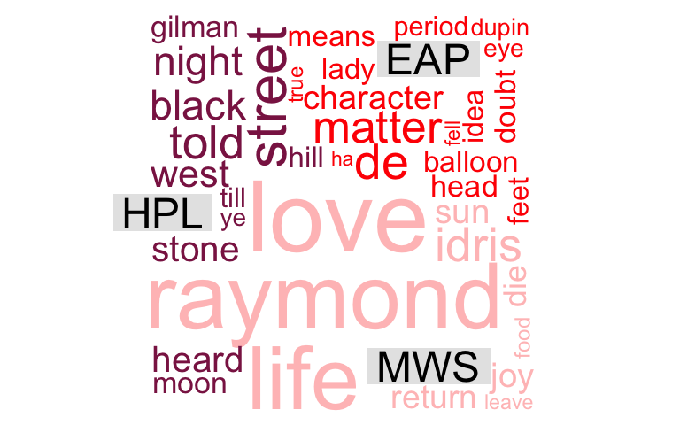
Another way to visualize the most frequent words by author is to use wordclouds. Wordclouds make it easy to spot differences, the importance of each word matches its font size and color.
par(mfrow = c(1,3), mar = c(0,0,0,0))
words_author <- get_common_words_by_author(x = spooky_trainining_tidy_1n,
author = "EAP",
remove.stopwords = TRUE)
mypal <- brewer.pal(8,"Spectral")
wordcloud(words = c("EAP", words_author$word),
freq = c(max(words_author$n) + 100, words_author$n),
colors = mypal,
scale=c(7,.5),
rot.per=.15,
max.words = 100,
random.order = F)
words_author <- get_common_words_by_author(x = spooky_trainining_tidy_1n,
author = "HPL",
remove.stopwords = TRUE)
mypal <- brewer.pal(8,"Spectral")
wordcloud(words = c("HPL", words_author$word),
freq = c(max(words_author$n) + 100, words_author$n),
colors = mypal,
scale=c(7,.5),
rot.per=.15,
max.words = 100,
random.order = F)
words_author <- get_common_words_by_author(x = spooky_trainining_tidy_1n,
author = "MWS",
remove.stopwords = TRUE)
mypal <- brewer.pal(8,"Spectral")
wordcloud(words = c("MWS", words_author$word),
freq = c(max(words_author$n) + 100, words_author$n),
colors = mypal,
scale=c(7,.5),
rot.per=.15,
max.words = 100,
random.order = F)
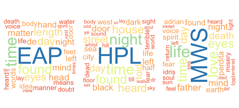 Most common words used by authors
From the word clouds, we can infer that EAP loves to use the words time, found, eyes, length, day, etc.HPL loves to use the words night, time, found, house, etc.MWS loves to use the words life, time, love, eyes, etc.
A comparison cloud can be used to compare the different authors. From the R documentation
‘Let p{i,j} be the rate at which word i occurs in document j, and p_j be the average across documents(∑ip{i,j}/ndocs). The size of each word is mapped to its maximum deviation ( max_i(p_{i,j}-p_j) ), and its angular position is determined by the document where that maximum occurs.’
See below the comparison cloud between all authors:
comparison_data <- spooky_trainining_tidy_1n %>%
dplyr::select(author, word) %>%
dplyr::anti_join(stop_words) %>%
dplyr::count(author,word, sort = TRUE)
comparison_data %>%
reshape2::acast(word ~ author, value.var = "n", fill = 0) %>%
comparison.cloud(colors = c("red", "violetred4", "rosybrown1"),
random.order = F,
scale=c(7,.5),
rot.per = .15,
max.words = 200)
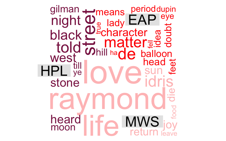 Comparison cloud between authors
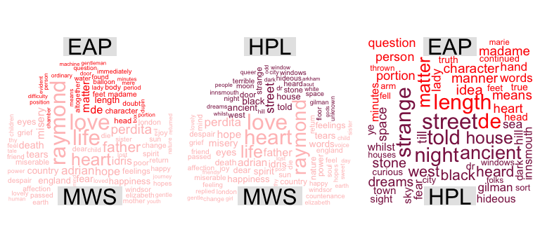
Below is the comparison clouds between the authors, two authors at any time.
par(mfrow = c(1,3), mar = c(0,0,0,0))
comparison_EAP_MWS <- comparison_data %>%
dplyr::filter(author == "EAP" | author == "MWS")
comparison_EAP_MWS %>%
reshape2::acast(word ~ author, value.var = "n", fill = 0) %>%
comparison.cloud(colors = c("red", "rosybrown1"),
random.order = F,
scale=c(3,.2),
rot.per = .15,
max.words = 100)
comparison_HPL_MWS <- comparison_data %>%
dplyr::filter(author == "HPL" | author == "MWS")
comparison_HPL_MWS %>%
reshape2::acast(word ~ author, value.var = "n", fill = 0) %>%
comparison.cloud(colors = c("violetred4", "rosybrown1"),
random.order = F,
scale=c(3,.2),
rot.per = .15,
max.words = 100)
comparison_EAP_HPL <- comparison_data %>%
dplyr::filter(author == "EAP" | author == "HPL")
comparison_EAP_HPL %>%
reshape2::acast(word ~ author, value.var = "n", fill = 0) %>%
comparison.cloud(colors = c("red", "violetred4"),
random.order = F,
scale=c(3,.2),
rot.per = .15,
max.words = 100)
 Comparison cloud between EAP, HPL, and MWS
Question: How many unique words are needed in the author dictionary to cover 90% of the used word instances?
words_cov_author_1 <- plot_word_cov_by_author(x = spooky_trainining_tidy_1n, author = "EAP")
words_cov_author_2 <- plot_word_cov_by_author(x = spooky_trainining_tidy_1n, author = "HPL")
words_cov_author_3 <- plot_word_cov_by_author(x = spooky_trainining_tidy_1n, author = "MWS")
gridExtra::grid.arrange(words_cov_author_1, words_cov_author_2, words_cov_author_3, nrow = 1)
 Detailed comparison cloud between EAP, HPL, and MWS
From the plot above we can see that for EAP and HPL provided corpus, we need circa 7500 words to cover 90% of word instance. While for MWS provided corpus, circa 5000 words are needed to cover 90% of word instances.
Question: Is there any commonality between the dictionaries used by the authors?
Are the authors using the same words? A commonality cloud can be used to answer this specific question, it emphasizes the similarities between authors and plot a cloud showing the common words between the different authors. It shows only those words that are used by all authors with their combined frequency across authors.
See below the commonality cloud between all authors.
comparison_data <- spooky_trainining_tidy_1n %>%
dplyr::select(author, word) %>%
dplyr::anti_join(stop_words) %>%
dplyr::count(author,word, sort = TRUE)
mypal <- brewer.pal(8,"Spectral") comparison_data %>%
reshape2::acast(word ~ author, value.var = "n", fill = 0) %>%
commonality.cloud(colors = mypal,
random.order = F,
scale=c(7,.5),
rot.per = .15,
max.words = 200)
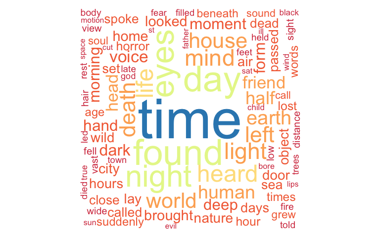 Frequency of word usage
Question: Can Word Frequencies be used to compare different authors?
First of all, we need to prepare the data calculating the word frequencies for each author.
word_freqs <- spooky_trainining_tidy_1n %>%
dplyr::anti_join(stop_words) %>%
dplyr::count(author, word) %>%
dplyr::group_by(author) %>%
dplyr::mutate(word_freq = n/ sum(n)) %>%
dplyr::select(-n)
Then we need to spread the author (key) and the word frequency (value) across multiple columns (note how NAs have been introduced for words not used by an author).
word_freqs <- word_freqs%>%
tidyr::spread(author, word_freq)
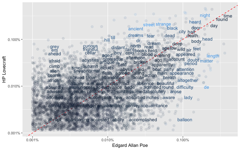
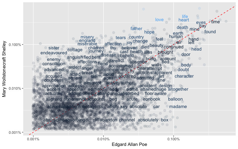
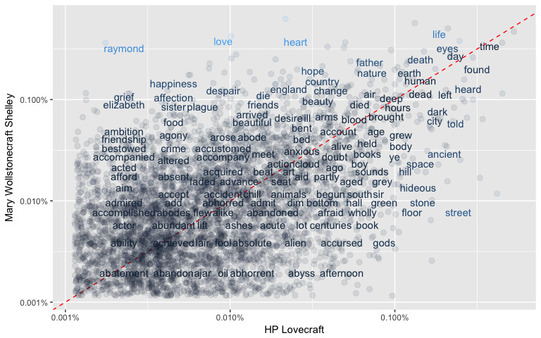
Let's start to plot the word frequencies (log scale) comparing two authors at a time and see how words distribute on the plane. Words that are close to the line (y = x) have similar frequencies in both sets of texts. While words that are far from the line are words that are found more in one set of texts than another.
As we can see in the plots below, there are some words close to the line but most of the words are around the line showing a difference between the frequencies.
# Removing incomplete cases - not all words are common for the authors
when spreading words to all authors - some will get NAs (if not used
by an author)
word_freqs_EAP_vs_HPL <- word_freqs %>%
dplyr::select(word, EAP, HPL) %>%
dplyr::filter(!is.na(EAP) & !is.na(HPL))
ggplot(data = word_freqs_EAP_vs_HPL, mapping = aes(x = EAP, y = HPL, color = abs(EAP - HPL))) +
geom_abline(color = “red”, lty = 2) +
geom_jitter(alpha = 0.1, size = 2.5, width = 0.3, height = 0.3) +
geom_text(aes(label = word), check_overlap = TRUE, vjust = 1.5) +
scale_x_log10(labels = scales::percent_format()) +
scale_y_log10(labels = scales::percent_format()) +
theme(legend.position = “none”) +
labs(y = “HP Lovecraft”, x = “Edgard Allan Poe”)
# Removing incomplete cases - not all words are common for the authors
when spreading words to all authors - some will get NAs (if not used
by an author)
word_freqs_EAP_vs_MWS <- word_freqs %>%
dplyr::select(word, EAP, MWS) %>%
dplyr::filter(!is.na(EAP) & !is.na(MWS))
ggplot(data = word_freqs_EAP_vs_MWS, mapping = aes(x = EAP, y = MWS, color = abs(EAP - MWS))) +
geom_abline(color = “red”, lty = 2) +
geom_jitter(alpha = 0.1, size = 2.5, width = 0.3, height = 0.3) +
geom_text(aes(label = word), check_overlap = TRUE, vjust = 1.5) +
scale_x_log10(labels = scales::percent_format()) +
scale_y_log10(labels = scales::percent_format()) +
theme(legend.position = “none”) +
labs(y = “Mary Wollstonecraft Shelley”, x = “Edgard Allan Poe”)
# Removing incomplete cases - not all words are common for the authors
# when spreading words to all authors - some will get NAs (if not used
# by an author)
word_freqs_HPL_vs_MWS <- word_freqs %>%
dplyr::select(word, HPL, MWS) %>%
dplyr::filter(!is.na(HPL) & !is.na(MWS))
ggplot(data = word_freqs_HPL_vs_MWS, mapping = aes(x = HPL, y = MWS, color = abs(HPL - MWS))) +
geom_abline(color = "red", lty = 2) +
geom_jitter(alpha = 0.1, size = 2.5, width = 0.3, height = 0.3) +
geom_text(aes(label = word), check_overlap = TRUE, vjust = 1.5) +
scale_x_log10(labels = scales::percent_format()) +
scale_y_log10(labels = scales::percent_format()) +
theme(legend.position = "none") +
labs(y = "Mary Wollstonecraft Shelley", x = "HP Lovecraft")
In order to quantify how similar/different these sets of word frequencies by author, we can calculate a correlation (Pearson for linearity) measurement between the sets. There is a correlation of around 0.48 to 0.5 between the different authors (see plot below).
word_freqs %>%
select(-word) %>%
cor(use="complete.obs", method="spearman") %>%
corrplot(type="lower",
method="pie",
diag = F)
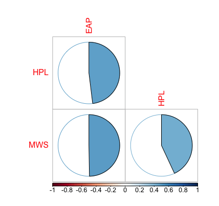 Correlation between EAP, HPL, and MWS
Get started with R programming with this free of cost course: Beginner R programming course.
References
[1] Kaggle challenge: Spooky Author Identification[2] “Text Mining in R – A tidy Approach” by J. Silge & D. Robinsons, O’Reilly 2017[3] “Regular Expressions, Text Normalization, and Edit Distance” draft chapter by D. Jurafsky & J. H . Martin, 2018
Appendix: Supporting functions
getNoExcerptsFor <- function(x, author){
sum(x$author == author)
}
getPercentageExcerptsFor <- function(x, author){
round((sum(x$author == author)/ dim(x)[1]) * 100, digits = 2)
}
get_xxx_length <- function(x, author, func){
round(func(x[x$author == author,]$len), digits = 2)
}
plot_common_words_by_author <- function(x, author, remove.stopwords = FALSE, greater.than = 90){
the_title = author
if(remove.stopwords){
x <- x %>% dplyr::anti_join(stop_words)
}
x[x$author == author,] %>%
dplyr::count(word, sort = TRUE) %>%
dplyr::filter(n > greater.than) %>%
dplyr::mutate(word = reorder(word, n)) %>%
ggplot(mapping = aes(x = word, y = n)) +
geom_col() +
xlab(NULL) +
ggtitle(the_title) +
coord_flip() +
theme_dark(base_size = 10)
}
get_common_words_by_author <- function(x, author, remove.stopwords = FALSE){
if(remove.stopwords){
x <- x %>% dplyr::anti_join(stop_words)
}
x[x$author == author,] %>%
dplyr::count(word, sort = TRUE)
}
plot_word_cov_by_author <- function(x,author){
words_author <- get_common_words_by_author(x, author, remove.stopwords = TRUE) words_author %>%
mutate(cumsum = cumsum(n),
cumsum_perc = round(100 * cumsum/sum(n), digits = 2)) %>%
ggplot(mapping = aes(x = 1:dim(words_author)[1], y = cumsum_perc)) +
geom_line() +
geom_hline(yintercept = 75, color = “yellow”, alpha = 0.5) +
geom_hline(yintercept = 90, color = “orange”, alpha = 0.5) +
geom_hline(yintercept = 95, color = “red”, alpha = 0.5) +
xlab(“no of ‘unique’ words”) +
ylab(“% Coverage”) +
ggtitle(paste(“% Coverage unique words -”, author, sep = “ “)) +
theme_dark(base_size = 10)
}
sessionInfo()
## R version 3.3.3 (2017-03-06)
## Platform: x86_64-apple-darwin13.4.0 (64-bit)
## Running under: macOS 10.13
##
## locale:
## [1] no_NO.UTF-8/no_NO.UTF-8/no_NO.UTF-8/C/no_NO.UTF-8/no_NO.UTF-8
##
## attached base packages:
## [1] stats graphics grDevices utils datasets methods base
##
## other attached packages:
## [1] bindrcpp_0.2 corrplot_0.84 wordcloud_2.5
## [4] RColorBrewer_1.1-2 gridExtra_2.3 dplyr_0.7.3
## [7] purrr_0.2.3 readr_1.1.1 tidyr_0.7.1
## [10] tibble_1.3.4 ggplot2_2.2.1 tidyverse_1.1.1
## [13] tidytext_0.1.3
##
## loaded via a namespace (and not attached):
## [1] httr_1.3.1 ddalpha_1.2.1 splines_3.3.3
## [4] jsonlite_1.5 foreach_1.4.3 prodlim_1.6.1
## [7] modelr_0.1.1 assertthat_0.2.0 highr_0.6
## [10] stats4_3.3.3 DRR_0.0.2 cellranger_1.1.0
## [13] yaml_2.1.14 robustbase_0.92-7 slam_0.1-40
## [16] ipred_0.9-6 backports_1.1.0 lattice_0.20-35
## [19] glue_1.1.1 digest_0.6.12 rvest_0.3.2
## [22] colorspace_1.3-2 recipes_0.1.0 htmltools_0.3.6
## [25] Matrix_1.2-11 plyr_1.8.4 psych_1.7.8
## [28] timeDate_3012.100 pkgconfig_2.0.1 CVST_0.2-1
## [31] broom_0.4.2 haven_1.1.0 caret_6.0-77
## [34] scales_0.5.0 gower_0.1.2 lava_1.5
## [37] withr_2.0.0 nnet_7.3-12 lazyeval_0.2.0
## [40] mnormt_1.5-5 survival_2.41-3 magrittr_1.5
## [43] readxl_1.0.0 evaluate_0.10.1 tokenizers_0.1.4
## [46] janeaustenr_0.1.5 nlme_3.1-131 SnowballC_0.5.1
## [49] MASS_7.3-47 forcats_0.2.0 xml2_1.1.1
## [52] dimRed_0.1.0 foreign_0.8-69 class_7.3-14
## [55] tools_3.3.3 hms_0.3 stringr_1.2.0
## [58] kernlab_0.9-25 munsell_0.4.3 RcppRoll_0.2.2
## [61] rlang_0.1.2 grid_3.3.3 iterators_1.0.8
## [64] labeling_0.3 rmarkdown_1.6 gtable_0.2.0
## [67] ModelMetrics_1.1.0 codetools_0.2-15 reshape2_1.4.2
## [70] R6_2.2.2 lubridate_1.6.0 knitr_1.17
## [73] bindr_0.1 rprojroot_1.2 stringi_1.1.5
## [76] parallel_3.3.3 Rcpp_0.12.12 rpart_4.1-11
## [79] tidyselect_0.2.0 DEoptimR_1.0-8 Written by Pier Lorenzo Paracchini
Want to build AI agents that can reason, plan, and execute autonomously?
Learn more